if (! require("tidyverse")) install.packages(
  pkgs = "tidyverse", repos = "http://cran.us.r-project.org"
)
if (! require("here")) install.packages(
  pkgs = "here", repos = "http://cran.us.r-project.org"
)
if (! require("tidytuesdayR")) install.packages(
  pkgs = "tidytuesdayR", repos = "http://cran.us.r-project.org"
)
if (! require("broom")) install.packages(
  pkgs = "broom", repos = "http://cran.us.r-project.org"
)
if (! require("circlize")) install.packages(
  pkgs = "circlize", repos = "http://cran.us.r-project.org"
)
if (! require("igraph")) install.packages(
  pkgs = "igraph", repos = "http://cran.us.r-project.org"
)9 Student mobility in Europe
NSC-R Tidy Tuesday November 2023
9.1 Introduction
In this workshop, Wim Bernasco explores a Tidy Tuesday dataset about the European Union Erasmus+ student mobility program. This dataset was used in the main Tidy Tuesday of week 10 in 2022. For more information on this data, including the codebook, see the RForDataScience GitHub registry.
In this workshop, the focus is on exploring, analyzing, and maybe visualizing student streams between countries. Different descriptive questions will be answered (Bernasco, 2022).
Here you find the link to the NSC-R Tidy Tuesday page.
9.2 Get started
Install uninstalled packages tidyverse, here and tidytuesdayR.
Load the required libraries
library(tidyverse)
library(broom)
library(here)
library(tidytuesdayR)
library(circlize)
library(igraph)
Load the datafile For information see
Note
The ‘participants’ field is a frequency weight!
Open the dataset
tuesdata <- tt_load(2022, week = 10)
Downloading file 1 of 1: `erasmus.csv`erasmus <- tuesdata$erasmusThere are two additional ‘helper’ datafiles used used in this script: country_names.csv: The full names and EU-status of the countries adjacency.csv : Pairs of countries that are adjacent (share borders)
I will address some of the following descriptive questions:
- How many students studied abroad?
- What are the top-10 receiving countries?
- What are the top-10 sending countries?
- Which are the 10 most frequent origin-destination country combinations?
- Are reverse flows (the flow from A to B and the flow from B to A) correlated?
The following modeling questions will be answered:
- How does total number of students from country A to country B depend on the total number of student from A and the total number of students from B?
- Do adjacent countries attract more or less students than non-adjacent countries?
If time permits some visualization questions will be answered:
- Are there some ways of visualizing mobility data?
9.3 Exploration and preparation
First we explore the data:
erasmus |> names() [1] "project_reference" "academic_year"
[3] "mobility_start_month" "mobility_end_month"
[5] "mobility_duration" "activity_mob"
[7] "field_of_education" "participant_nationality"
[9] "education_level" "participant_gender"
[11] "participant_profile" "special_needs"
[13] "fewer_opportunities" "group_leader"
[15] "participant_age" "sending_country_code"
[17] "sending_city" "sending_organization"
[19] "sending_organisation_erasmus_code" "receiving_country_code"
[21] "receiving_city" "receiving_organization"
[23] "receiving_organisation_erasmus_code" "participants" erasmus |> glimpse()Rows: 164,635
Columns: 24
$ project_reference <chr> "2014-1-AT02-KA347-000139", "2014-~
$ academic_year <chr> "2014-2015", "2014-2015", "2014-20~
$ mobility_start_month <chr> "2014-11", "2014-11", "2014-11", "~
$ mobility_end_month <chr> "2014-11", "2014-11", "2014-11", "~
$ mobility_duration <dbl> 1, 1, 1, 1, 1, 1, 1, 1, 1, 1, 1, 1~
$ activity_mob <chr> "National youth meetings", "Nation~
$ field_of_education <chr> "? Unknown ?", "? Unknown ?", "? U~
$ participant_nationality <chr> "AT", "AT", "AT", "AT", "AT", "AT"~
$ education_level <chr> "??? - ? Unknown ?", "??? - ? Unkn~
$ participant_gender <chr> "Female", "Female", "Female", "Mal~
$ participant_profile <chr> "Learner", "Learner", "Learner", "~
$ special_needs <chr> "No", "No", "No", "No", "No", "No"~
$ fewer_opportunities <chr> "Yes", "Yes", "Yes", "Yes", "Yes",~
$ group_leader <chr> "No", "No", "No", "No", "No", "No"~
$ participant_age <dbl> 13, 14, 15, 14, 15, 15, 16, 17, 18~
$ sending_country_code <chr> "AT", "AT", "AT", "AT", "AT", "AT"~
$ sending_city <chr> "Dornbirn", "Dornbirn", "Dornbirn"~
$ sending_organization <chr> "bOJA - Bundesweites Netzwerk Offe~
$ sending_organisation_erasmus_code <chr> "-", "-", "-", "-", "-", "-", "-",~
$ receiving_country_code <chr> "AT", "AT", "AT", "AT", "AT", "AT"~
$ receiving_city <chr> "Dornbirn", "Dornbirn", "Dornbirn"~
$ receiving_organization <chr> "bOJA - Bundesweites Netzwerk Offe~
$ receiving_organisation_erasmus_code <chr> "-", "-", "-", "-", "-", "-", "-",~
$ participants <dbl> 2, 3, 3, 4, 2, 2, 1, 3, 1, 2, 1, 2~erasmus |> count(participants)# A tibble: 99 x 2
participants n
<dbl> <int>
1 1 118352
2 2 22804
3 3 8756
4 4 4642
5 5 2572
6 6 1775
7 7 1125
8 8 874
9 9 668
10 10 502
# ... with 89 more rowsFirst check number of rows
erasmus |> dim()[1] 164635 24Number of rows after ‘expansion’. Expansion expands a frequency-weighted datafile to a regular file where each row represents a single student exchange trip.
erasmus |>
  uncount(participants) |>
  dim()
[1] 309751 23From which countries do participants come?
erasmus |>
  count(sending_country_code)
# A tibble: 54 x 2
sending_country_code n
<chr> <int>
1 AL 132
2 AM 127
3 AT 3484
4 AZ 54
5 BA 83
6 BE 3279
7 BG 4412
8 BY 69
9 CY 1886
10 CZ 6086
# ... with 44 more rowsTo which country do participants go?
erasmus |>
  count(receiving_country_code)
# A tibble: 34 x 2
receiving_country_code n
<chr> <int>
1 AT 3451
2 BE 4008
3 BG 4120
4 CY 1981
5 CZ 6107
6 DE 17000
7 DK 1484
8 EE 3637
9 EL 2042
10 ES 11188
# ... with 24 more rowsAdd names to the codes. There are several options to do this. - Option 1: Explicit in-script recoding
erasmus |>
  mutate(sending_country_name =
           case_when(sending_country_code == "AT" ~ "Austria",
                     sending_country_code == "BE" ~ "Belgium",
                     sending_country_code == "BG" ~ "Bulgaria",
                     sending_country_code == "CY" ~ "Cyprus",
                     sending_country_code == "CZ" ~ "Czechia",
                     sending_country_code == "DE" ~ "Germany",
                     sending_country_code == "DK" ~ "Denkmark"
                     # .........
           )) |>
  count(sending_country_name)
# A tibble: 8 x 2
sending_country_name n
<chr> <int>
1 Austria 3484
2 Belgium 3279
3 Bulgaria 4412
4 Cyprus 1886
5 Czechia 6086
6 Denkmark 1426
7 Germany 17155
8 <NA> 126907- Option 2: Join with look-up table in a separate CSV file
country_labels <- read_csv(here("C:/Users/Gebruiker/Desktop/TidyTuesday/TT_20221115/country_names.csv"))erasmus |>
left_join(country_labels,
by=c("receiving_country_code" = "country_code")) |>
rename(receiving_country_name = country_name,
receiving_country_status = country_status)# A tibble: 164,635 x 26
project_ref~1 acade~2 mobil~3 mobil~4 mobil~5 activ~6 field~7 parti~8 educa~9
<chr> <chr> <chr> <chr> <dbl> <chr> <chr> <chr> <chr>
1 2014-1-AT02-~ 2014-2~ 2014-11 2014-11 1 Nation~ ? Unkn~ AT ??? - ~
2 2014-1-AT02-~ 2014-2~ 2014-11 2014-11 1 Nation~ ? Unkn~ AT ??? - ~
3 2014-1-AT02-~ 2014-2~ 2014-11 2014-11 1 Nation~ ? Unkn~ AT ??? - ~
4 2014-1-AT02-~ 2014-2~ 2014-11 2014-11 1 Nation~ ? Unkn~ AT ??? - ~
5 2014-1-AT02-~ 2014-2~ 2014-11 2014-11 1 Nation~ ? Unkn~ AT ??? - ~
6 2014-1-AT02-~ 2014-2~ 2014-12 2014-12 1 Nation~ ? Unkn~ AT ??? - ~
7 2014-1-AT02-~ 2014-2~ 2014-12 2014-12 1 Nation~ ? Unkn~ AT ??? - ~
8 2014-1-AT02-~ 2014-2~ 2014-12 2014-12 1 Nation~ ? Unkn~ AT ??? - ~
9 2014-1-AT02-~ 2014-2~ 2014-12 2014-12 1 Nation~ ? Unkn~ AT ??? - ~
10 2014-1-AT02-~ 2014-2~ 2014-12 2014-12 1 Nation~ ? Unkn~ AT ??? - ~
# ... with 164,625 more rows, 17 more variables: participant_gender <chr>,
# participant_profile <chr>, special_needs <chr>, fewer_opportunities <chr>,
# group_leader <chr>, participant_age <dbl>, sending_country_code <chr>,
# sending_city <chr>, sending_organization <chr>,
# sending_organisation_erasmus_code <chr>, receiving_country_code <chr>,
# receiving_city <chr>, receiving_organization <chr>,
# receiving_organisation_erasmus_code <chr>, participants <dbl>, ...Combining some of the above transformations we created a clean file
labeled_erasmus_full <-
  erasmus |>
  # Keep only a subset of columns/variables
  select(sending_country_code, receiving_country_code,
         participant_gender, academic_year, activity_mob, participants) |>
  # insert names of receiving countries by linking to country codes
  left_join(country_labels,
            by=c("receiving_country_code" = "country_code")) |>
  # make sure the column names are clear
  rename(receiving_country_name = country_name,
         receiving_country_status = country_status) |>
  # insert names of sending countries by linking to country codes
  left_join(country_labels,
            by=c("sending_country_code" = "country_code")) |>
  # make sure the column names are clear
  rename(sending_country_name = country_name,
         sending_country_status = country_status) |>
  # exclude countries outside EU and with no affiliation to EU
  filter(sending_country_status %in% c("EU", "EFTA", "UK", "Candidate"),
         receiving_country_status %in% c("EU", "EFTA", "UK", "Candidate")) |>
  # exclude the (many!) within-country exchanges
  filter(sending_country_code != receiving_country_code) |>
  # Only international mobility program
  filter(activity_mob == "Transnational youth meetings") |>
  # Every row becomes an individual international student trip
  uncount(participants)
9.4 Descriptive questions
How many students are there?
labeled_erasmus_full |>
  dim()
[1] 15693 9Where did they come from?
labeled_erasmus_full |>
  count(sending_country_name) |>
  print(n=Inf)
# A tibble: 36 x 2
sending_country_name n
<chr> <int>
1 Albania 169
2 Austria 565
3 Belgium 662
4 Bulgaria 526
5 Croatia 323
6 Cyprus 121
7 Czechia 531
8 Denmark 296
9 Estonia 292
10 Finland 307
11 France 622
12 Germany 1314
13 Greece 483
14 Hungary 473
15 Iceland 25
16 Ireland 225
17 Italy 1098
18 Latvia 386
19 Liechtenstein 6
20 Lithuania 411
21 Luxembourg 166
22 Malta 58
23 Montenegro 27
24 Netherlands 630
25 North Macedonia 185
26 Norway 133
27 Poland 837
28 Portugal 468
29 Romania 745
30 Serbia 343
31 Slovakia 370
32 Slovenia 268
33 Spain 819
34 Sweden 495
35 Turkey 553
36 United Kingdom 761Visualization as a bar graph
labeled_erasmus_full |>
  count(sending_country_name) |>
  ggplot() +
  geom_col(aes(x=sending_country_name, y=n))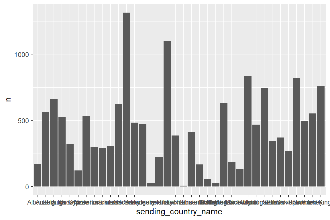
With vertical labels labels
labeled_erasmus_full |>
  count(sending_country_name) |>
  ggplot() +
  geom_col(aes(x=sending_country_name, y=n)) +
  theme(axis.text.x = element_text(angle = 90, vjust = 0.5, hjust=1))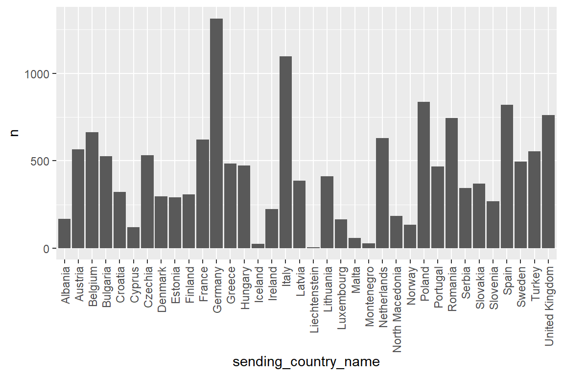
Order by frequency.
labeled_erasmus_full |>
  count(sending_country_code) |>
  arrange(-n) |>
    # Converting character variable to factor variable
    mutate(sending_country_code=factor(sending_country_code,
                                     levels = unique(sending_country_code),
                                     ordered = T)) |>
  ggplot() +
  geom_col(aes(x=sending_country_code, y=n)) +
  theme(axis.text.x = element_text(angle = 90, vjust = 0.5, hjust=1))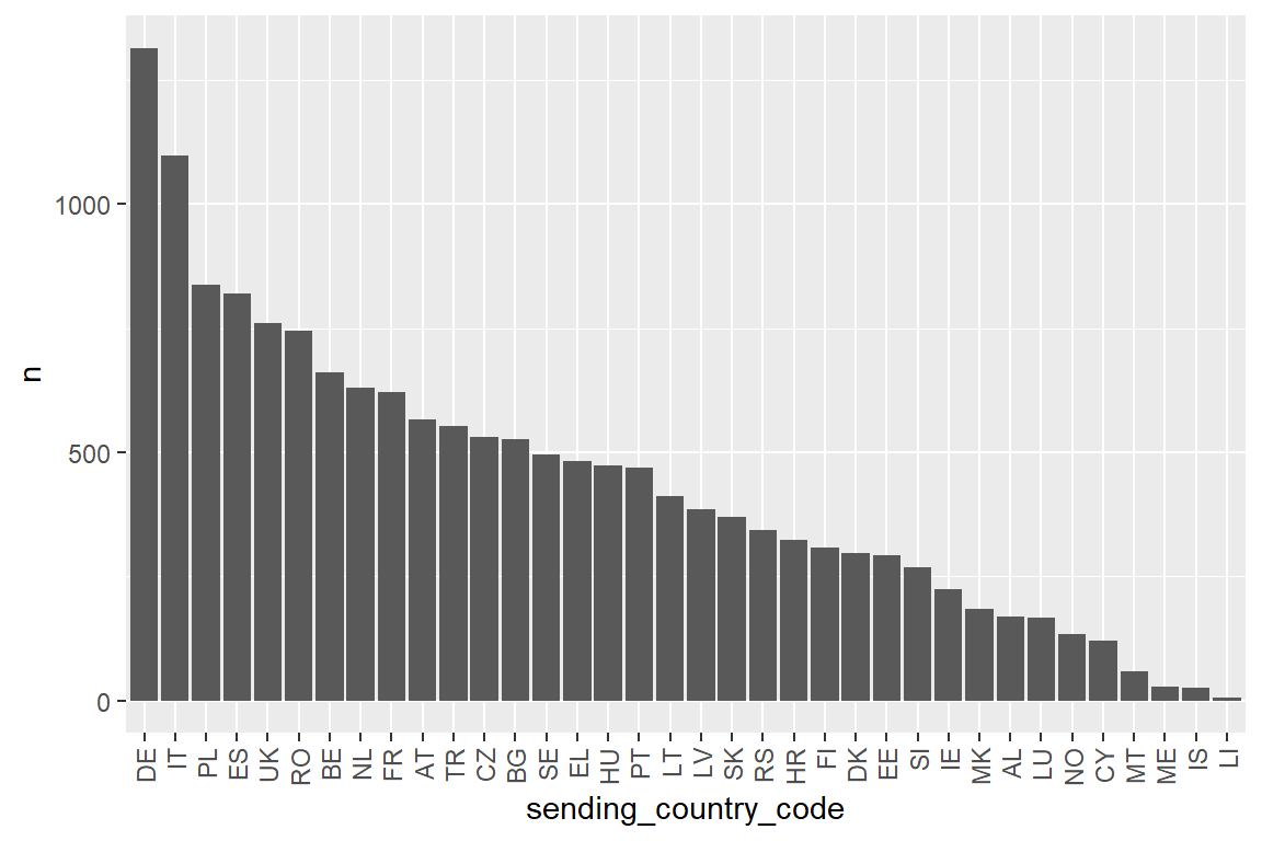
Where did they go to?
labeled_erasmus_full |>
  count(receiving_country_name) |>
  arrange(-n) |>
  print(n=Inf)
# A tibble: 31 x 2
receiving_country_name n
<chr> <int>
1 France 2403
2 Belgium 1428
3 Spain 1204
4 Germany 1095
5 Italy 1017
6 Netherlands 765
7 Luxembourg 607
8 Estonia 524
9 Czechia 518
10 Lithuania 495
11 Austria 485
12 United Kingdom 483
13 Greece 444
14 Romania 423
15 Turkey 371
16 Slovenia 355
17 Croatia 343
18 Denmark 340
19 Poland 340
20 Portugal 296
21 Norway 286
22 Sweden 250
23 Cyprus 214
24 Ireland 186
25 Latvia 165
26 Malta 163
27 Bulgaria 149
28 Hungary 116
29 North Macedonia 111
30 Slovakia 67
31 Finland 50labeled_erasmus_full |>
count(receiving_country_name) |>
arrange(-n) |>
print(n=Inf)# A tibble: 31 x 2
receiving_country_name n
<chr> <int>
1 France 2403
2 Belgium 1428
3 Spain 1204
4 Germany 1095
5 Italy 1017
6 Netherlands 765
7 Luxembourg 607
8 Estonia 524
9 Czechia 518
10 Lithuania 495
11 Austria 485
12 United Kingdom 483
13 Greece 444
14 Romania 423
15 Turkey 371
16 Slovenia 355
17 Croatia 343
18 Denmark 340
19 Poland 340
20 Portugal 296
21 Norway 286
22 Sweden 250
23 Cyprus 214
24 Ireland 186
25 Latvia 165
26 Malta 163
27 Bulgaria 149
28 Hungary 116
29 North Macedonia 111
30 Slovakia 67
31 Finland 50Let us visualise this also, vertical and ordered.
labeled_erasmus_full |>
  count(receiving_country_code) |>
  arrange(-n) |>
  mutate(receiving_country_code=factor(receiving_country_code,
                                       levels = unique(receiving_country_code),
                                       ordered = T)) |>
  ggplot() +
  geom_col(aes(x=receiving_country_code, y=n)) +
  theme(axis.text.x = element_text(angle = 90, vjust = 0.5, hjust=1))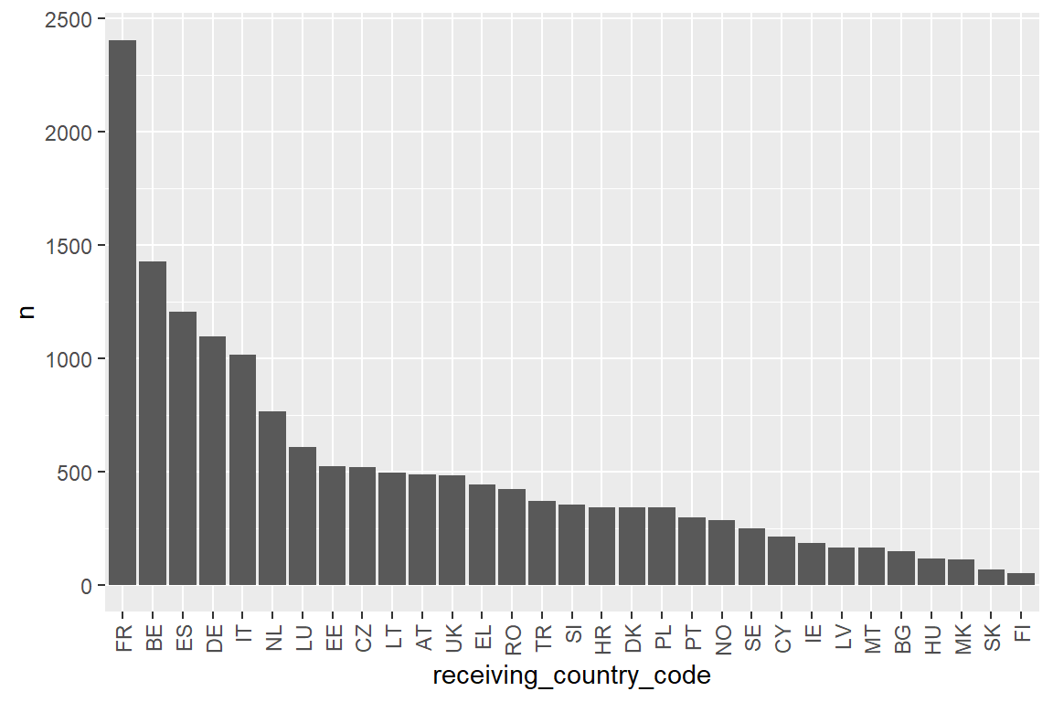
Top 10 Where did they go to.
labeled_erasmus_full |>
  count(receiving_country_name) |>
  arrange(-n) |>
  head(n=10)
# A tibble: 10 x 2
receiving_country_name n
<chr> <int>
1 France 2403
2 Belgium 1428
3 Spain 1204
4 Germany 1095
5 Italy 1017
6 Netherlands 765
7 Luxembourg 607
8 Estonia 524
9 Czechia 518
10 Lithuania 495Top 10 Where did they come from
labeled_erasmus_full |>
  count(sending_country_name) |>
  arrange(-n) |>
  head(n=10)
# A tibble: 10 x 2
sending_country_name n
<chr> <int>
1 Germany 1314
2 Italy 1098
3 Poland 837
4 Spain 819
5 United Kingdom 761
6 Romania 745
7 Belgium 662
8 Netherlands 630
9 France 622
10 Austria 565Top 10 origin-destination combinations
labeled_erasmus_full |>
  count(sending_country_name, receiving_country_name) |>
  arrange(-n) |>
  head(n=10)
# A tibble: 10 x 3
sending_country_name receiving_country_name n
<chr> <chr> <int>
1 Germany France 305
2 Italy France 268
3 Germany Belgium 235
4 Belgium France 198
5 Italy Spain 170
6 Spain France 149
7 United Kingdom France 131
8 Spain Italy 123
9 Poland France 122
10 France Belgium 120# Intermezzo
(Cartesian product = cross-product = all combinations)
Tiny dataset of team members
::: {.cell}
```{.r .cell-code}
team_members <- tibble(name = c( "Alex", "Asier", "Franziska", "Sam", "Wim"))
# Tiny datset of available days
sessions <- tibble(day = c("Monday", "Tuesday", "Thursday")):::
Make all combinations of team members and available days
full_join(team_members, sessions, by = as.character())# A tibble: 15 x 2
name day
<chr> <chr>
1 Alex Monday
2 Alex Tuesday
3 Alex Thursday
4 Asier Monday
5 Asier Tuesday
6 Asier Thursday
7 Franziska Monday
8 Franziska Tuesday
9 Franziska Thursday
10 Sam Monday
11 Sam Tuesday
12 Sam Thursday
13 Wim Monday
14 Wim Tuesday
15 Wim ThursdaySame results, but more transparent code.
thanks to Nick van Doormaal for this suggestion
expand_grid(team_members, sessions)# A tibble: 15 x 2
name day
<chr> <chr>
1 Alex Monday
2 Alex Tuesday
3 Alex Thursday
4 Asier Monday
5 Asier Tuesday
6 Asier Thursday
7 Franziska Monday
8 Franziska Tuesday
9 Franziska Thursday
10 Sam Monday
11 Sam Tuesday
12 Sam Thursday
13 Wim Monday
14 Wim Tuesday
15 Wim Thursdayfull_join(team_members, team_members, by = as.character()) |>
filter(name.x != name.y)# A tibble: 20 x 2
name.x name.y
<chr> <chr>
1 Alex Asier
2 Alex Franziska
3 Alex Sam
4 Alex Wim
5 Asier Alex
6 Asier Franziska
7 Asier Sam
8 Asier Wim
9 Franziska Alex
10 Franziska Asier
11 Franziska Sam
12 Franziska Wim
13 Sam Alex
14 Sam Asier
15 Sam Franziska
16 Sam Wim
17 Wim Alex
18 Wim Asier
19 Wim Franziska
20 Wim Sam
Create all possible combinations of sending and receiving country names.

::: {.cell}

```{.r .cell-code}
possible_mobility_names <-
  full_join(country_labels, country_labels,
            by = as.character()) |>
  select(sending_country_name   = country_name.x,
         receiving_country_name = country_name.y,
         sending_country_code   = country_code.x,
         receiving_country_code = country_code.y) |>
  filter(sending_country_name != receiving_country_name)
:::
Erasmus student mobility flows including zero flows
flows_erasmus_full_zeros <-
  labeled_erasmus_full |>
  group_by(sending_country_name, receiving_country_name) |>
  # Origin, destination, count
  count() |>
  rename(exchanges = n) |>
  # join with all combinations to include zero-flow pairs
  right_join(possible_mobility_names) |>
  # change the NAs (= zero-flow) into 0
  replace_na(list(exchanges=0))
Number of exchanges frequencies reversed: 581 zero flows, 37 1-person flow
flows_erasmus_full_zeros |>
  ungroup() |>
  count(exchanges) |>
  arrange(exchanges) |>
  print(n=40)
# A tibble: 98 x 2
exchanges n
<int> <int>
1 0 581
2 1 37
3 2 37
4 3 48
5 4 35
6 5 42
7 6 30
8 7 32
9 8 29
10 9 19
11 10 28
12 11 20
13 12 27
14 13 14
15 14 18
16 15 20
17 16 15
18 17 15
19 18 13
20 19 15
21 20 16
22 21 10
23 22 13
24 23 14
25 24 9
26 25 13
27 26 7
28 27 7
29 28 7
30 29 13
31 30 8
32 31 9
33 32 4
34 33 7
35 34 4
36 35 4
37 36 6
38 37 6
39 38 4
40 39 3
# ... with 58 more rowsLet us make a histogram of this distribution
flows_erasmus_full_zeros |>
  ggplot() +
  geom_histogram(aes(x=exchanges), binwidth = 5)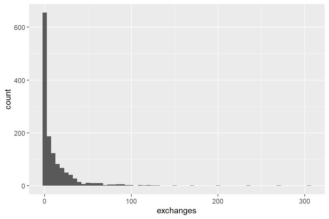
reverse_flows_erasmus_full_zeros <-
  flows_erasmus_full_zeros |>
  rename(sending_country_name = receiving_country_name,
         receiving_country_name = sending_country_name,
reverse_exchanges = exchanges)full_join(flows_erasmus_full_zeros, reverse_flows_erasmus_full_zeros,
by = (c("sending_country_name", "receiving_country_name"))) |>
ungroup() |>
select(exchanges, reverse_exchanges) |>
cor() |>
as_tibble()# A tibble: 2 x 2
exchanges reverse_exchanges
<dbl> <dbl>
1 1 0.463
2 0.463 1 This scatterplot is by design symetric in the diagonal
full_join(flows_erasmus_full_zeros, reverse_flows_erasmus_full_zeros,
          by = (c("sending_country_name", "receiving_country_name"))) |>
  ungroup() |>
  select(exchanges, reverse_exchanges) |>
  ggplot() +
  geom_point(aes(y=exchanges, x=reverse_exchanges) )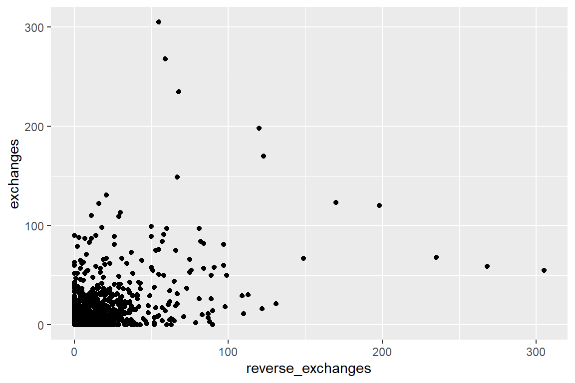
9.5 Modeling
Read the neighbor relations between countries
adjacency <- read_csv(here("C:/Users/Gebruiker/Desktop/TidyTuesday/TT_20221115/adjacency.csv")) |>
  rename(sending_country_name = country_name,
         receiving_country_name = neighbor) |>
  # mark the rows that indicate shared borders
  mutate(adjacent = 1) |>
  # merge with the data that include all possible mobility streams
  right_join(possible_mobility_names,
             by=c("sending_country_name","receiving_country_name")) |>
  # Set non-adjacent to 0
  mutate(adjacent = replace_na(adjacent, 0))
model_data <-
flows_erasmus_full_zeros |>
inner_join(adjacency,
by = c("sending_country_name","receiving_country_name")) |>
group_by(sending_country_name) |>
# total outflow from country
mutate(outflow = sum(exchanges)) |>
group_by(receiving_country_name) |>
# total inflow into country
mutate(inflow = sum(exchanges)) Number of student exchanges from A to B as a function of total numbers of outgoing students from A and of total numbers of visiting students in B
model_01 <- lm(formula = exchanges ~  inflow + outflow ,          ,
               data = model_data)
tidy(model_01)
# A tibble: 3 x 5
term estimate std.error statistic p.value
<chr> <dbl> <dbl> <dbl> <dbl>
1 (Intercept) -12.2 0.942 -13.0 2.49e- 36
2 inflow 0.0281 0.00100 27.9 1.63e-135
3 outflow 0.0285 0.00161 17.7 2.55e- 63glance(model_01)# A tibble: 1 x 12
r.squared adj.r.s~1 sigma stati~2 p.value df logLik AIC BIC devia~3
<dbl> <dbl> <dbl> <dbl> <dbl> <dbl> <dbl> <dbl> <dbl> <dbl>
1 0.448 0.447 17.5 539. 2.98e-172 2 -5703. 11415. 11436. 408538.
# ... with 2 more variables: df.residual <int>, nobs <int>, and abbreviated
# variable names 1: adj.r.squared, 2: statistic, 3: devianceAdd adjacency
model_02 <- lm(formula = exchanges ~  inflow + outflow + adjacent,
               data = model_data)
tidy(model_02)
# A tibble: 4 x 5
term estimate std.error statistic p.value
<chr> <dbl> <dbl> <dbl> <dbl>
1 (Intercept) -12.9 0.881 -14.7 2.03e- 45
2 inflow 0.0274 0.000939 29.1 1.27e-144
3 outflow 0.0265 0.00151 17.5 3.93e- 62
4 adjacent 23.0 1.64 14.0 9.76e- 42glance(model_02)# A tibble: 1 x 12
r.squared adj.r.s~1 sigma stati~2 p.value df logLik AIC BIC devia~3
<dbl> <dbl> <dbl> <dbl> <dbl> <dbl> <dbl> <dbl> <dbl> <dbl>
1 0.519 0.518 16.4 478. 1.36e-210 3 -5612. 11233. 11259. 355879.
# ... with 2 more variables: df.residual <int>, nobs <int>, and abbreviated
# variable names 1: adj.r.squared, 2: statistic, 3: devianceStudents appear to fancy visiting nearby countries abroad!
9.6 Visualization
Visualization 1: Chord diagram (using library circlize)
Full country names
flows_erasmus_full_zeros |>
  filter(exchanges > 0) |>
  arrange(-exchanges) |>
  chordDiagram()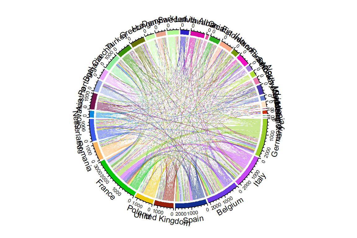
Use the 2-letter abbreviations of countries here.
flows_erasmus_full_zeros |>
  filter(exchanges > 0) |>
  arrange(-exchanges) |>
  # without ungroup() the .._country_name columns will
  # be retained
  ungroup() |>
  select(sending_country_code, receiving_country_code,
         exchanges) |>
  chordDiagram()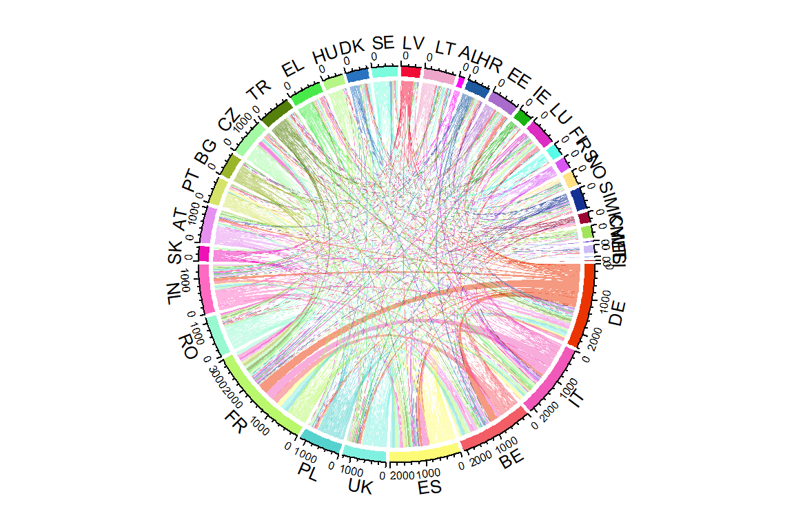
Only flows over 100
flows_erasmus_full_zeros |>
  filter(exchanges > 100) |>
  arrange(-exchanges) |>
  ungroup() |>
  select(sending_country_code, receiving_country_code,
         exchanges) |>
  chordDiagram()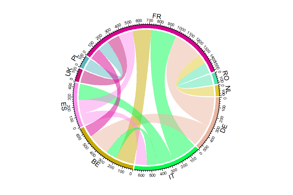
Visulaization 2: Network representation We can also represent the countries as nodes in a network, with the student flows representing the links between them. Use package igraph here.
flows_erasmus_full_zeros |>
  filter(exchanges > 100) |>
  graph_from_data_frame(directed = TRUE,
                      vertices=country_labels) |>
  plot(vertex.size=5)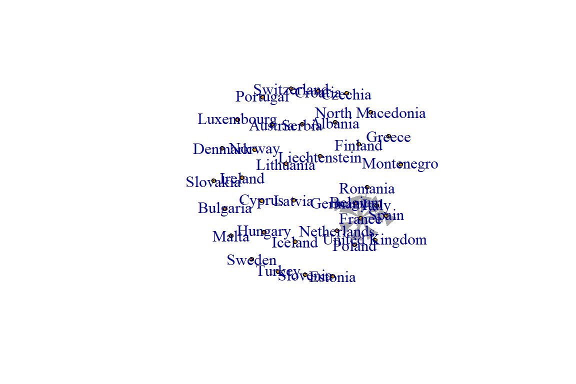
No isolates
flows_erasmus_full_zeros |>
filter(exchanges > 75) |>
graph_from_data_frame(directed = TRUE) |>
plot(vertex.size=5)
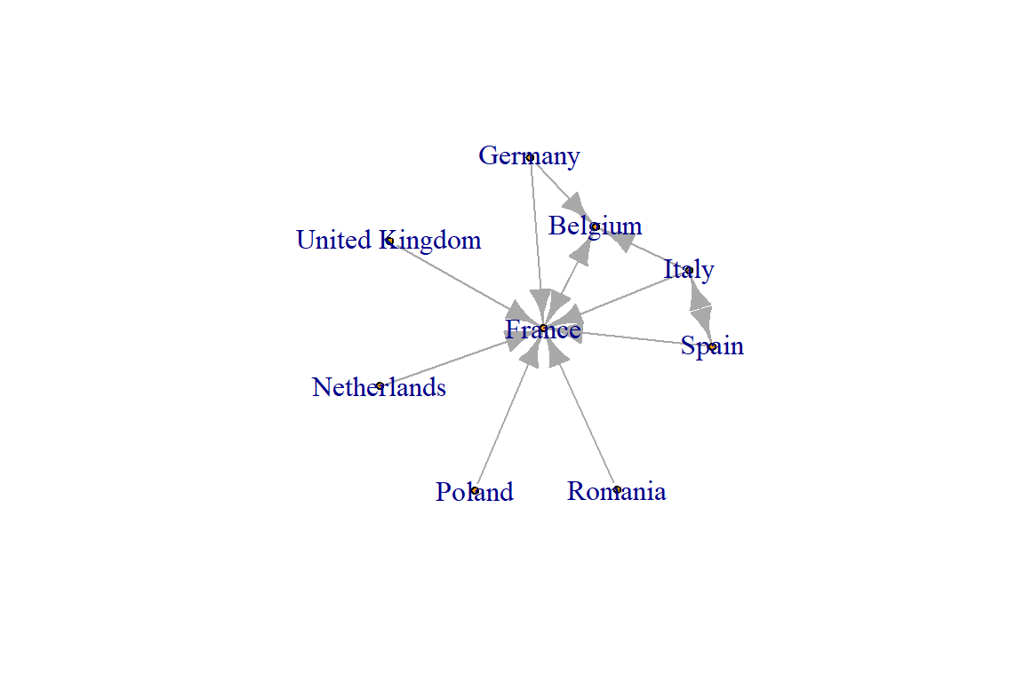
flows_erasmus_full_zeros |>
filter(exchanges > 100) |>
graph_from_data_frame(directed = TRUE) |>
plot(vertex.size=5)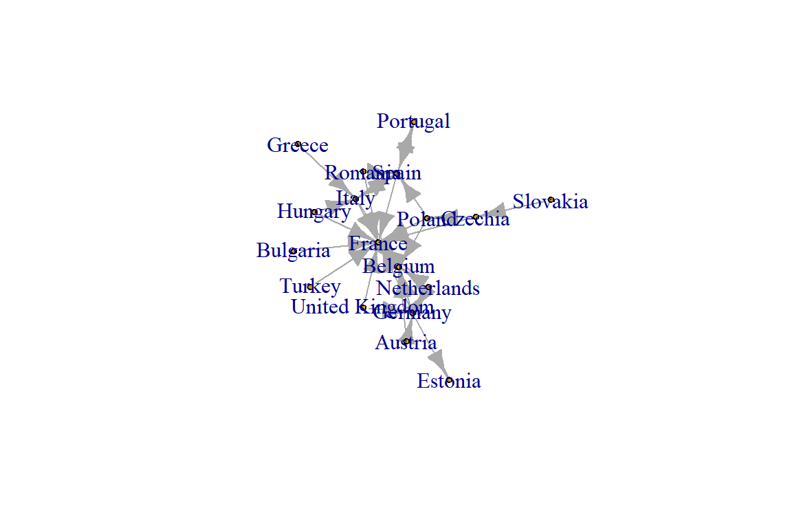
For alternative methods of visualizing mobility while maintaining the geographic relations, see Andrew Wheeler’s 2015 paper in Cartography and Geographic Information Science, at (behind paywall), here
9.7 References
Bernasco, W. (2022, November). NSC-R Workshops: NSC-R Tidy Tuesday. NSCR. Retrieved from https://nscrweb.netlify.app/posts/2022-11-15-nsc-r-tidy-tuesday/